Internet-Based Teaching and Learning in a Mid-Size
Honors Multivariable Calculus Course
Thomas F. Banchoff
Thomas_Banchoff@brown.edu
Mathematics Department
Brown University
Providence, RI 02912
U.S.A.
Abstract
At the 2005 international
symposium, Enhancing University Mathematics at KAIST
in Daejeon, Korea, we reported on our ten-year experience
of teaching geometry and calculus courses at all levels
using the Internet both for communication and for
demonstrations [B1] At the 2007 ATCM conference in Taipei,
we presented an example of an interactive article on
Critical Points and Curvature based on these courses and
this student-developed software [B2]. The purpose of
this article is to update those two reports and to present
evidence that interactive Internet-based courses can
enhance teaching and learning at different
scales. The primary examples come from a
course at Brown University in the fall semester of 2008 on
honors multivariable calculus for a class of 66 students,
twice the number as in previous classes. An extensive
questionnaire at the conclusion of that class provides
comparative data that validate the effectiveness of some
earlier modifications and suggest new directions for
pedagogical research.
This report contains four sections:
-
1—Summary of Features of the Tensor for
Internet-Based Teaching and Learning
-
2—The Two-Dimensional Table of Contents and
Improvements in Laboratory Software
-
3—Examples of Student Work Using the Tensor and
Demonstration Software
-
4—Assessment and Future Directions Based on
Comparison of Questionnaire Results
1—Summary of Features of the Tensor for
Internet-Based Teaching and Learning
Several key features of our approach have been
developed primarily in relatively small classes of
approximately 30 students. This past
semester, 66 students signed up for that same course so
the scale was different. This
necessitated rethinking several aspects of our
courseware, some of which were readily adaptable to a
larger group and several of which open new research
questions.
Math 35 has two 80-minute lectures per week, a format
more suited to an honors course where students
generally have more background and a longer attention
span than to a standard course where three 50-minute
classes per week spreads out the new ideas in a way
that is more easily
digestible. For a class of 30
students, it is possible to assign and respond to two
assignments per week, with responses posted online in
the Tensor. The first assignment is
given out on the afternoon of the Tuesday class and is
to be handed in online by Wednesday night at 10
p.m. This short assignment gives the
students a chance to see if they have understood the
lecture material well enough to solve problems, as well
as to think about the new ideas that are going to be
presented on Thursday. The
benefit for the teacher is intermediate feedback that
indicates whether or not it is safe to continue with an
idea that most students have followed up to that
point. It also flags certain points
of confusion that can be cleared up at the beginning of
the Thursday lecture. After that
lecture, a more substantial problem set is posted, due
on Monday morning by 3 a.m. so that the online
responses are ready to be read and commented on by the
instructor (and assistants if available) by Monday
afternoon in preparation for the upcoming
week. Up to the time the
assignment is due, only the student can view his or her
work and the instructor comments, and after the due
time, all students in the class can read the responses
of others, together with comments, unless some
submissions have been designated as
“private” (a feature instituted as a result
of requests on questionnaires of previous
courses).
The Tensor is the piece of communication software where
all the responses are collected. By default only the
last five assignments are presented in a matrix, and
selecting "Show All Assignments" will present all the
entries of all students over the course of the
semester. Selecting a week or other heading in the
leftmost column with open a matrix for that assignment,
with problems listed on the leftmost column and student
user id initials across the top. Selecting any entry
shows the students response and the comment of the
instructor. A square in the matrix is red if the most
recent response came from the student and green if the
most recent activity is a comment from the instructor.
Mathematical autobiographies are automatically private,
i.e. so they only available to be read by the
instructors of that class.
One (unintended) consequence of the ability to respond
to comments is that some students engage in a dialogue
until they get all the aspects of a problem
correct. While this is certainly beneficial to
the student, it involves extra time on the part of the
instructor. Even without such back-and-forth
online discussion, the practice of providing responses
before the beginning of the next class involves a
serious time commitment on the part of the instructor.
Before class on Tuesday, students are expected to read
the comments on their work as well as the Solution Key,
usually a compilation of exemplary (or at least
interesting) responses transferred from student
responses by the instructor, often together with
additional commentary. It is
possible for students to enter comments about the work
of others in the class, although this aspect is not
often used unless the instructor specifically requests
it on certain occasions.
This commitment on the part of the students and the
instructor is substantial and labor
intensive. For 30 students, it is
possible to keep up the effort; for 66, it is far more
difficult. There are two major
differences that emerged in the course in the fall of
2008: First of all, students still
were faithful and appreciative about reading comments
on their own work, but fewer took the opportunity to
look at the work of other students in the Tensor,
relying instead on the selected responses collected in
the Solution Key. Secondly, to a
much greater extent than previously, the course
employed group work. Each of these
aspects was treated in the end-of-course questionnaire,
and the assessment based on these data appears in the
final section of this paper, where we also refer to
suggestions and comments about the privacy option and
the Solution Key.
One aspect that did not change was student use of the
demonstration software in assignments and in the
interactive laboratories. Under the
Resources Menu in the course webpage, there is a link
to the interactive laboratories developed using the
senior thesis of David Eigen, a math-CS concentrator
who devised the program for generating Java applets for
use in a variety of mathematics courses at Brown. The
Math 35 page includes a basic tutorial for using the
Java demos. Each section of the labs starts with a
labeled picture and a plus sign that can be selected to
see more information about the concept illustrated in
the demo as well as a button that opens a Java applet.
The student can explore a particular phenomenon,
entering in new data and manipulating the images. In
order to share what he or she has discovered or
created, the student can save the applet tag and enter
it into a homework answer or a discussion. Anyone
who opens the button that appears in the document will
enter the program exactly where the student left off.
The instructor or another student can then make
comments, sometimes illustrated by a modification of
the given applet.
A difference from earlier instances this course is the
variety of techniques used by students to enter their
responses in the Tensor. As a result
of student suggestions and requests from earlier
courses, we included “shortcuts” to make it
easier for students to type mathematical expression in
html. A number of students continued
to use this feature throughout the semester, while
others chose to use more sophisticated software,
primarily LaTeX. We also made it
more straightforward for students to upload their
written work and many chose to submit their work this
way, both in assignments and in
examinations. It is probably
worthwhile repeating the comment made in previous
papers that students can immediately type their work
into the Tensor without any significant preparation or
instruction, once they know how to enter exponents and
subscripts and a few mathematical symbols for
inequalities and the square root.
For example, in the first assignment after the first
lecture, Thunwa Theerakarn typed in
his answer to the following problem:
Problem: What is the range of the function f(x,y)
= x2 + 2bxy + y2, defined for all
(x,y)? (The answer will depend on b. Try to cover all
possible cases.)
Thunwa Theerakarn at 2008-09-07
17:07:43.0
To find the range of the function
f(x,y) = x2 + 2bxy + y2, for any y,
we can choose t = x + by. Then f(x,y) =
t2 + (1- b2) y2
Case |b| ≤ 1 :
Since t2 ≥ 0 and (1-
b2) y2 ≥ 0, we have f(x,y) ≥
0.
Range is all positive real numbers and
zero.
Case |b| < 1 :
Since t2 can be any positive
real number and (1- b2) y2 can be any
negative real number, range of f(x,y) is all real
numbers.
Another feature of the online course that worked well
but required extra effort was giving take-home
examinations. There were two
mid-term exams, each scheduled for five days, and a
one-week final examination.
Such exams routinely include a number of standard
problems, as well as others that are less specifically
defined and more open to interpretation and
exploration. It takes a long time to
grade such examinations, since the instructor is
responsible for all such grading.
Some examples of more complex problems that can be
assigned in such examinations are given in the next
section. In the author’s
viewpoint, these more challenging and open-ended
problems can be the most rewarding aspect of the class,
for the students as well as the
instructor. They give students a
chance to display a range of thoughtful responses,
often leading to multiple approaches to problems that
can be collected in the Solution
Key.
Examples of such open problems and student responses
appear in the third section of this report.
2—The Two-Dimensional Table of Contents and
Improvements in Laboratory Software
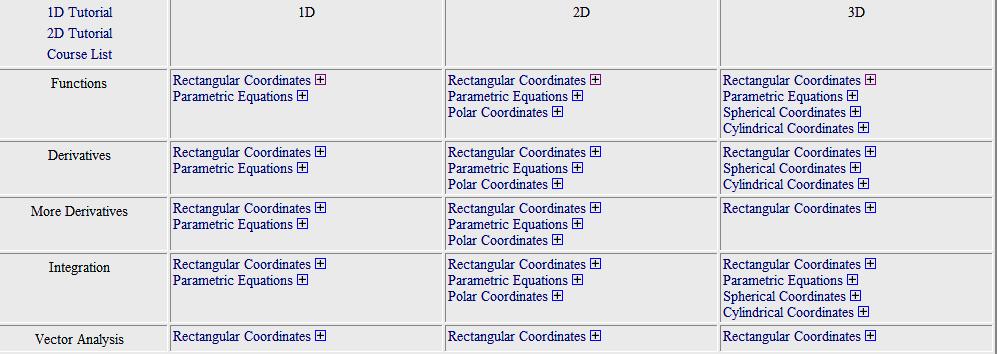
A new feature of our laboratory software is a more
explicit two-dimensional table of
contents. Calculus topics appear in
the rows of a matrix, with three columns, for functions
of one, two, or three variables. At
any point, a student can navigate from a topic in
two-variable calculus “to the left” to
recall the corresponding one-variable topic in a way
suitable for generalization, or “to the
right” to see further generalizations for
functions of three and more
variables. We continue to look for
ways to make this access tool even more powerful and
engaging.
Each topic listed in the two-dimensional table of
contents is in a column according to its dimension. At
any time, a student can move “leftward”
from a laboratory demonstration on two-variable
calculus to the corresponding demonstration for
one-variable calculus, or “rightward” to
see how the notion will be extended to functions of
three or more variables.
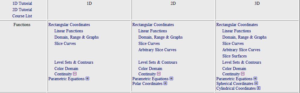
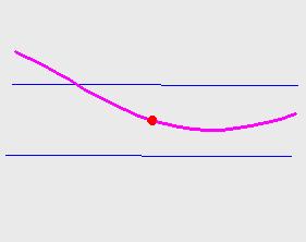
We illustrate this setup with two examples. The
first involves continuity, a notion that many students
understand only imperfectly after a first course in
calculus, especially from a geometric point of view
that can be particularly helpful in calculus of two
variables. We interpret continuity as a
challenge-response situation, and in any number of
variables, the process is the same. Given a
function f(x) of one variable and a point x0
of the domain, the challenger chooses a pair of
horizontal lines at distance ε from y =
f(x0) and asks if the domain can be
restricted to points with distance less than δ
from x0 so that the graph over that
restricted domain lies between the two horizontal
lines. If every challenge can be met, then the
function is continuous at x0. In the
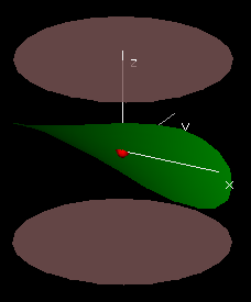
case of a function of two variables, the challenge is
the same, except that there are two horizontal planes
at distance ε from the plane z =
f(x0,y0) and the responder has to
choose δ so small that the graph over the disc of
radius δ centered at
(x0,y0) lies between the
planes.
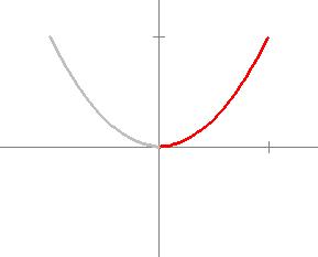
Another example refers to the author’s paper in
Volume 2, Number 2 of eJMT. Critical
points of a function of one variable can be visualized
by coloring the graph of a function f(x) red if the
derivative f’(x) is positive.
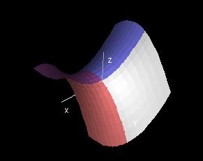
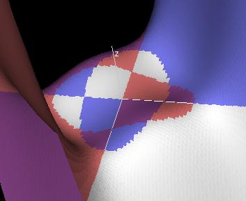
Similarly critical points of a function of two
variables can be visualized by coloring the graph of a
function f(x,y) red if fx(x,y) is positive,
blue if fy(x.y) is positive, and purple if
both are positive.
An example appears in the interactive article [B1]
concerning the topic of critical
points. Students are familiar
with Rolle’s theorem for a function f(x) of a
single variable, stating that such a continuous
function defined over an interval a
≤
b must have an interior local maximum or
minimum or both if f(a) = f(b).
To generalize this, consider a continuous
function f(x,y) defined on a region D bounded
by a curve C on which the function f is
constant. The conclusion is
that there must be a local maximum or a local
minimum or both in the interior of
D. If the function of one
variable is differentiable, then the
derivative of f must be zero at any interior
local maximum or minimum so the tangent line
is horizontal there. For a
function of two variables, all partial
derivatives at in interior local maximum or
minimum must be zero and the tangent planes at
such points must be
horizontal. Students can
then be challenged to state and
prove generalizations of
the Mean Value Theorem, where a differentiable
function f(x,y) coincides with a linear
function L(x,y) = ax + by + c on the boundary
C curve of a disc domain D.
More complex questions deal with the number of
critical points of various types for functions
that are assumed to be non-negative on a
domain and zero on the
boundary. In the case of
one variable, if the critical points are
isolated maxima and minima, then the number of
maxima is one greater than the number of
minima. For the
corresponding two-dimensional theorem, if all
critical points are m0 local
minima, m1 ordinary saddles, and
m2 local maxima, then students can
explore and come up with the conjecture that
m2 – m1 +
m0 = 1, a powerful and important
result popularized by Marston Morse and
reported in [M].
Interactive Laboratories: Under the Resources Menu
in the course webpage, there is a link to the
interactive laboratories developed using the senior
thesis of David Eigen, a math-CS concentrator who
devised the program for generating Java applets for
use in a variety of mathematics courses at Brown.
The Math 35 page includes a basic tutorial for
using the Java demos. Each section of the labs
starts with a labeled picture and a plus sign that
can be selected to see more information about the
concept illustrated in the demo as well as a button
that opens a Java applet. The student can explore a
particular phenomenon, entering in new data and
manipulating the images. In order to share what he
or she has discovered or created, the student can
save the applet tag and enter it into a homework
answer or a discussion. Anyone who opens the
button that appears in the document will enter the
program exactly where the student left off. The
instructor or another student can then make
comments, sometimes illustrated by a modification
of the given applet.
3—Examples of Student Work Using the Tensor
and Demonstration Software
Examples of such investigations from the Tensor
appear in the work of Soravit Changpinyo and Thunwa
Theerakarn, both students from Thailand in my
honors multivariable class.
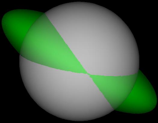
Problem: Analyze the function f(x,y) =
xy(1 - x
2 - y
2) showing the graph
of the function together with its zero contour, and
identify the critical points of the function. What is
the maximum value taken on by the function on the
domain consisting of all (x,y) with x
2 +
y
2 ≤ 4?
Soravit Changpinyo solves part (a) really well:
f(x,y) =
xy(1-x2-y2)
f(x,y) = 0 when x=0 or y =0 or
x2 + y2 = 1
Its zero contour is along the light
blue curve, two linear lines and a circle.
fx(x,y) = xy(-2x) +
(1-x2-y2)y = -3yx2 + y
– y3
fy(x,y) = xy(-2y) +
(1-x2-y2)x = -3xy2 + x
– x3
fx(x,y) = -3yx2 + y –
y3 = 0
y(1-3x2-y2) = 0
(1) y = 0
or
(2)
3x2+y2 = 1
fy(x,y) = -3xy2 + x –
x3 = 0
x(1-3y2-x2) = 0
(3) x = 0
or
(4)
3y2+x2 = 1
The critical points are all (x,y) such that
fx(x,y) = 0 and fy(x,y) = 0
They could be represented by the intersections of two
ellipses (3x2 + y2 = 1 and
3y2 + x2 = 1), the intersections
of two lines (the x-axis and the y-axis), and the
intersections of the line and the ellipse of different
colors.
Solve for (x,y) from (1) and (3); (0,0)
Solve for (x,y) from (1) and (4); (-1,0), (1,0)
Solve for (x,y) from (2) and (3); (0,1), (0,-1)
Solve for (x,y) from (2) and (4); (0.5,0.5),
(-0.5,0.5), (0.5,-0.5), (-0.5,-0.5)
The critical points are (0,0,0), (-1,0,0),
(1,0,0), (0,1,0), (0,-1,0), (0.5,0.5,0), (-0.5,0.5,0),
(0.5,-0.5,0), (-0.5,-0.5,0).
0 <= x2 + y2 <= 4
-3 <= 1 - x2 - y2 <= 1
(|x|-|y|)2 = x2 - 2|xy| +
y2 >= 0
2|xy| >= 4
|xy| <= 2
-2 <= xy <= 2
xy and 1 - x2 - y2 must have
the same sign so their product is positive.
if both xy and 1 - x2 - y2 are
positive, the possible maximum of the product is (1)(2)
= 2.
if both xy and 1 - x2 - y2 are
negative, the possible maximum of the product is
(-2)(-3) = 6.
The maximum value taken on by the function on the
domain consisting of all (x,y) with x2 +
y2 <= 4 is 6.
The demo below shows that there are two maximum
points. Both of them satisfy x2 +
y2 = 4.
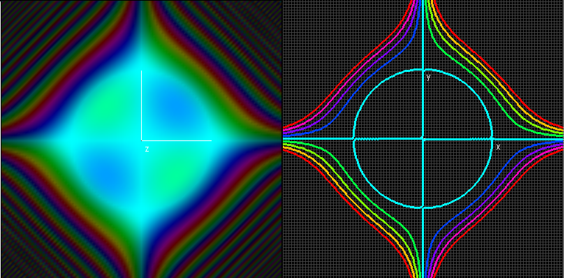
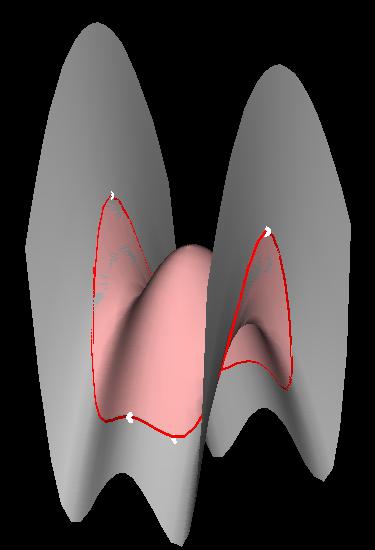
Problem:
What can you say about the function g(x,y) =
x4 –
6x2y2 +
y4 .
(Standard Hint: look at the
graph.)
Thunwa Theerakarn
used standard Macintosh graphing hardware to produce
images that he included in his assignments
:
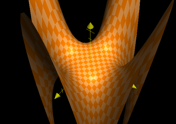
Graph of g(x,y) = g(x,y) = x4 –
6x2y2 +
y4
With plane cut through g(x,y) = 0. The view is from
above looking down to xy-plane.
We will see that the plane divides the surface into 8
symmetrical pieces, 4 above and 4 below.
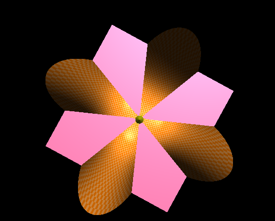
Make a conjecture that g(x,y) can be written in
cos(4θ) form in polar coordinates.
Consider
g(x,y) = x4 –
6x2y2 +
y4 .
= r4cos4θ -
6r4cos2
θsin2θ +
r4sin4θ
= [r4cos4θ -
2r4cos2θsin2θ
+ r4sin4θ] -
4r4cos2
θsin2θ
= [r4[cos2θ
-sin2θ]2] -
r4sin2 (2θ)
= r4[cos2 (2θ)2
- r4sin2 (2θ)
= r4cos(4θ)
Therefore, zero contour level is
lines cos(4θ) = 0, that is, the lines
θ = π/8 , 3π/8 ,
5π/8 , 7π/8, 9π/8, 11π/8, 13π/8,
15π/8.
It might be interesting
to some readers to look at the responses of these two
students to the initial questionnaire for the course:
In Soravit’s Mathematical Autobiography, written
the first day of the course, he states: “There
are three things I expect from this class. The first
thing is challenging stuff. Math that’s too easy
isn’t fun. Another thing is a strong foundation
in calculus that will ease my learning in computer
science. Lastly, I would like to learn about math not
only from the instructors, but also from my peers. I
know everyone is exceptionally
talented.” He indicated in his
questionnaire that my course had been recommended to
him by Saran Ahuja, a member of the Thai Mathematical
Olympiad team when he was a student at the Montford
School in Chiangmai, and one of the top students in my
course in Honors Linear Algebra during his first
semester at Brown three years ago.
Thunwa writes “At
the end of my high school years, I won a Thai
Government scholarship to study in the United States
from undergrad to Ph.D. The scholarship requires me to
earn degree on Applied Mathematics and I will have to
work in a university in Thailand for twice as time I
will have spent here. This course will be hard -
I know. Somebody told me I should not start first year
in college with a hard course. But... there's so much
to learn, and I'm willing to learn it. As always, it
will be challenging, fun, and beautiful.
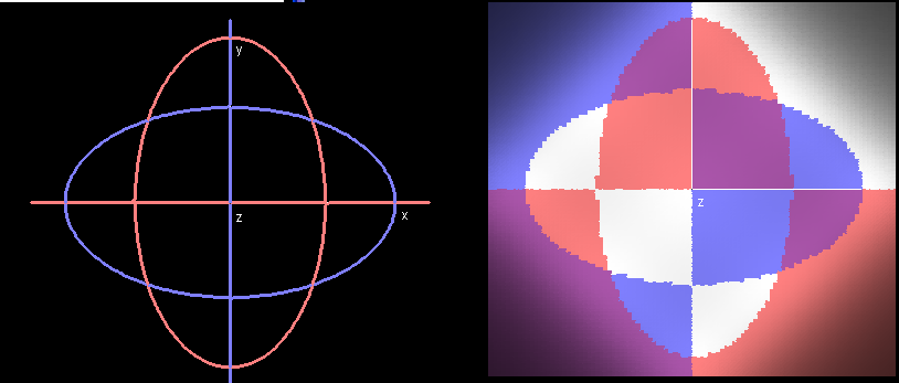
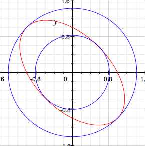
Problem: Find
the points of the ellipse x
2 + xy +
y
2 = 1 closest to the origin and furthest
from the origin by finding the critical points of
f(x,y) = x
2 + y
2 on the ellipse.
(See the Hint to recall the procedure for Lagrange
multipliers.)
Solution to
Problem:
Let g(x,y) = x2 + xy + y2
f(x,y) = x2 + y2
Consider the minimum and maximum of f(x,y) on level
curve g(x,y) = 1
Using Lagrange multipliers,
∇f(x,y) = λ ∇g(x,y)
∇f(x,y) = (2x,2y)
∇g(x,y) = (2x+y,2y+x)
2x = λ(2x+y) and 2y = λ(2y+x)
That is 2x/(2x + y) = 2y/(2y + x)
that is x2 = y2
Case x = y
from g(x,y) we get that x2 + x(x) +
x2 = 1
That is 3x2 = 1
x = 1/√3
(x,y) = (1/√3,1/√3) ,
(-1/√3,-1/√3)
f(x,y) = x2 + y2 = 2/3
Case x = -y
From g(x,y) = 1, we get that x2 = 1
That is x = ±1
(x,y) = (1,-1) , (-1,1)
f(x,y) = x2 + y2 = 2
Therefore, g(x,y) closest to the origin at (x,y) =
(1/√3,1/√3) , (-1/√3,-1/√3) and
furthest at
(x,y) = (1,-1), (-1,1).
Problem: Find
the critical points of the function f(x,y,z) =
x
2 + y
2 +
z
2 on the ellipsoid
x
2 + y
2/4+ z
2/9 = 1
and indicate whether they are maxima or minima or
other.
Here is a demo intended to give some inspiration.
Changing r will alter the radius of an expanding
sphere, representing the contour surfaces of f(x,y,z).
What happens when the sphere and the ellipsoid
intersect?
Solution to
Problem:
f(x,y,z) = x2 + y2 +
z2
Let g(x,y,z) = x2 + y2/4 +
x2/9
Consider the critical points of f(x,y,z) on the level
set of g(x,y,z) = 1
Using Lagrange multipliers
∇f(x,y,z) =
λ∇g(x,y,z)
That is (2x+2y+2z) = λ(2x+y/2+2z/9)
implies
2x = λ2x
2y = λy/2
2z = λ2z/9
That is
x = 0 or λ = 1
y = 0 or λ = 4
z = 0 or λ = 9
Consider that in each case, λ cannot be the
same constant. Therefore, two of {x,y,z} have to equal
zero in each case.
When x=0, z=0, y=±2
f(x,y,z) = 4
When x=0,y=0 , z=±3
f(x,y,z) = 9
When y=0, z=0 , x=±1
f(x,y,z) = 1
Therefore, (0,0,±3) are maxima, (±1,0,0)
are minima and (0,±2,0) are critical points but
not maxima or minima.
At the critical points, the gradient vectors of f
and g are parallel
Critical Points at Level f(x,y,z) = 2
We take our final illustration from one of the
problems on the midterm examination. The first
examination in the course took place four weeks after
the start of the semester. The Midterm
Examination was a take-home test over a period of six
days. It consisted of ten problems, each with two
or three parts, and students were permitted to use
notes and books and computers, as well as all the
material on the class website, but they all agreed that
no one would consult anyone else, either in person or
electronically.
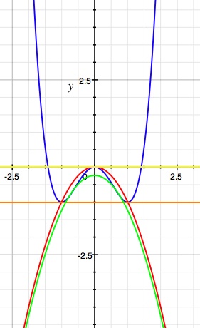
The first problem required students to identify the
critical points of a polynomial function f(x,y) =
x4 – 2x2 –
y2 and to find the maximum and minimum
values on a disc of radius R centered at the origin,
where the result depended on R.
The last part of the problem was subtle enough to
test the ingenuity of most students. William
Fallon devised a demonstration that was particularly
useful in seeing how the image of a disk of radius R
changed with R,
Gili Kriger was able to construct a two-dimensional
graphic showing five different functions of R on the
same diagram, from which it was possible to read off
the required maxima and minima, and to provide
algebraic justification for the listing of
results.
4—Assessment and Future
Directions Based on Comparison of Questionnaire
Results
Recent proposals to the Division of Undergraduate
Education of the National Science Foundation have
placed special emphasis on developing effective
assessments of the teaching and learning aspects of the
project, particularly in the dissemination phase.
Potential users of the technology need to know the
results of our experience, and the ways in which we
have modified the course, the technology, and the
assessment instruments, so that they can determine
whether and how this approach might be adapted to their
needs and the needs of their students and
institutions.
Course
evaluation data have been collected in more than twenty
courses using this approach, mostly at Brown University
but also at Yale University, the University of Notre
Dame, UCLA, and at the University of Georgia, both in
the Mathematics department and in the College of
Education. In 2004, we redesigned our
questionnaires with the help of a professional market
researcher who specializes in analysis of qualitative
data. She has developed a method for systematically
analyzing the data using a form of content analysis
which enables us to summarize and display our results,
course by course as well as for the same course across
semesters and teaching situations (i.e., different
teachers, different schools). These data collection
techniques and methods of analyses represent a
substantial improvement over our earlier assessment
efforts.
For each
course, the data were aggregated into
question-by-question spreadsheets; responses for each
question part, or sub-question, were coded (positive,
neutral, and negative using a three-point scale) and
displayed next to the individual verbatim response.
Finally, summary tables were generated for each
question by sub-questions. In this method of analysis,
some comments within verbatim responses could be
highlighted for making summary points in the data
tables, and for use in reports and
presentations.
(Verbatim comments
were only reported for students who had handed in a
written statement giving the instructor permission to
use submitted work in presentations and
reports.)
Examining
coded verbatim responses for each question reveals
patterns in students’ responses within a course.
Summary tables of codes by question and sub-question
yields the more substantive analysis, and results for
the same question or sub-parts of a question can be
compared across time. Examining the data in these
several systematic ways establishes a basis for
deciding how to adapt and improve the teaching
technology and interactive process for students and the
teaching situation for the
instructor.
Response
rates for the two courses were comparable; in
Fall 2004, 39 of 60 students completed course
evaluations (65%), and in Fall 2008, course
evaluations were received from 54 of 63 students who
completed the course
(86%).
In 2004, the
questionnaire included nine questions (with up to four
sub-parts), covering: 1) online assignments, 2)
solution keys and hints 3) online student interaction
4) online communication with instructors 5) timing of
assignments 6) examinations 7) textbook 8)
visualization software (“demos”), and 9) an
additional open-ended question allowing for general
comments. In 2008, question 7
was altered since there was no specific text for the
course, and a tenth question was added concerning the
policy of working in groups for the bi-weekly homework
assignments (a new procedure introduced in
2008).
In 2004,
students submitted their course evaluations online
after they completed classes and before completing
their final exam, while in 2008, students submitted
their course evaluations online just after completing a
final take-home exam, with the understanding that the
questionnaires would only be read after the grades had
been determined.
Analysis
of the Question on Comfort Level for Sharing Work
Online
The value of
this assessment method can be illustrated with an
analysis of responses to an important question we asked
about our teaching and learning approach, namely how
“comfortable” students are with opening
their work to other students online. This element of
viewing the work of their classmates, and instructor
comments is central to our model of teaching and
learning. We also asked if students if
their attitudes had changed over time.
In the 2004 questionnaire, some
students expressed discomfort at having their work on
assignments and examinations, as well as instructor
comments (but not grades) available for others to
read. In subsequent courses, the software was
modified so that students are given the option to
designate any particular response
“private”, so only readable by
instructors. Responses to the analysis of other
questions have also led to modifications and
refinements; we expect this to continue during the
dissemination phase of our
project.
Table 1. Learning from other Students
Honors
Multivariable Calculus
| a. How often did you look at the work of other students? |
Fall
2004 |
|
Fall
2008 |
| (Base: # Respondents) |
(39)
# |
|
(54)
# |
“Usually”
“Sometimes”/“occasionally”
“Rarely”/“hardly ever”
“Never”
No answer |
14
15
10
0
0
|
|
7
19
21
6
1 |
| b. Did you look at the work of some students more often than others? If so, how did you decide whose work to look at? |
| (Base: # Respondents) |
(39)
# |
|
(54)
# |
“No”
“Yes”
No answer |
8
30
1 |
|
12
36
6 |
| c. How comfortable were you with having your homework available for other students to read? |
| (Base: # Respondents) |
(39)
# |
|
(54)
# |
“Okay”/“no problem”
“Some reservation [but] no objection”
“Not comfortable”
No answer |
34
5
0
0
|
|
36
8
3
7 |
| d. How comfortable were you with having your exams available for other students to read? |
| (Base: # Respondents) |
(39)
# |
|
(54)
# |
“Okay”/“no problem”
“Some reservation [but] no objection”
“Not comfortable”
No answer |
30
9
0
0 |
|
28
12
9
5
|
Several students
reported changes in their attitudes over time. Most
interesting is the student who said:
"In the
beginning I really did not like the system of
reading other student homework.
It made me feel really nervous and
exposed and it made me want to leave problems
blank rather than to put in an incorrect answer.
As the semester progressed I realized what a
useful tool it could be and I started reading
other people's hw responses more and more and
felt more comfortable with mine being read."
Another student
addressed motivation:
"It didn't
really bother me that other people could look at
my work, either at the beginning or the end of
the semester. Sometimes I felt bad about
the quality of the work that I handed in and I
might have preferred that others not look at it,
but it didn't concern me enough to make me want
to change the system and the motivation to do a
better job probably didn't hurt
either."
As the numbers
indicate, some students felt differently about
exams:
"I think I am more
self-conscious about my exams. At first I didn't mind
so much, but now I am beginning to think that there
should be some element of privacy with exams, or a way
to choose to have your exam available or not".
A
counter-intuitive response
was:
"I have
always been self-conscious about having work of
mine open to criticism, so I was slightly
uncomfortable (about the homework being
available)" but "On exams, I was
able to put more time into refining my answer, so
I didn't mind having people see
that."
Analysis of the Questions on Group Work for
Assignments
A major change in
the communication aspect of the course is the
requirement that students participate in homework
groups for their bi-weekly assignments, resulting in a
manageable 20 or so responses instead of
66. Comfort levels on making homework
responses public rose slightly, although most students
reported sharing primarily within the group rather than
reading other entries in the Tensor.
A number of students appreciated selecting certain
student answers for the Solution Key for each
assignment. There was still some
dissatisfaction with making examination answers
available for everyone in the class to
read. On the basis of this
information, we will alter the software so that it will
be possible for a student to designate the totality of
his or her examination responses as private, rather
than having to make this designation on each separate
question.
Table 2. Sample Groups A and
H
|
Briefly, describe the way that you worked [in your homework group]:
|
| |
|
|
10.a
|
10.b
|
10.c
|
|
Group
|
ID
|
|
a) Who was in your homework group? How
often did you meet in person? How many
attended in-person sessions? How did
your meetings change over the
semester?
|
b) What problems, if any, did you
experience with the group process? Any
suggestions for improving
it?
|
c) How comfortable were you working in the
group? Did your feelings
change?
|
|
A
|
amc
|
2
|
kmd, a person in my dorm. We met about twice a week, always in person.
|
OK
|
None really.
|
OK
|
It was very helpful for me at time. We sometimes thought up some clever stuff together.
|
|
A
|
kmd
|
2
|
I was in a group with amc. ... we would meet the night it was due and clear up any problems that we had. Usually ... about a half hour or so (occasionally much longer if we had lots of questions). As the course progressed I found that I typically was the one who was typing up the problems which was fine because that was how I like to do the problems anyway.
|
+/-
|
I felt as though groups can benefit certain people more than others. Typically one person will have more problems with the homework than others which means that one person will spend most of the time explaining to other people which is less beneficial for them.
|
OK
|
I felt very comfortable working in the group.
|
|
H
|
mlw
|
5
|
For the majority of the assignments I worked with [names] ... since I ... worked a lot with [names] in physics class and we worked well together. We usually met pretty consistently every Sunday and Wednesday in person to do the homework.
|
OK
|
The group worked great for me.
|
OK
|
In the beginning I was not excited about having to do the homework in groups, but it turned out to be very useful. Especially when the problems were conceptually difficult it was really beneficial having lots of people thinking about it and eventually talking it out rather than potentially getting stuck not starting a lot more problems. Having to explain our thinking seemed to make everyone grasp the material better since its a lot easier to write faulty logic than talk other people through it.
|
|
H
|
adp
|
5
|
Me, [names] ... We met once for each assignment we were allowed to do in groups, but not otherwise. Everyone showed up, and we'd split up the problems but everyone would check everyone else's work
|
OK
|
None except that it made the non-group process seem more difficult
|
OK
|
consistently comfortable
|
|
H
|
bal
|
5
|
[names] ... were in my group. We met in person for almost every homework assignment towards the end of the semester. Not that frequently at the beginning. We all attended the sessions.Our meetings became more productive over the semester.
|
OK
|
The geographic organization of groups is a good starting point. It's much easier to work with people who you live near.
|
OK
|
I was more comfortable towards the end of the semester. The first group meeting was awkward and we didn't work as well since we were just getting to know one another.
|
|
H
|
rpp
|
5
|
My core homework group consisted of [names] ... and myself. We met twice a week and usually worked out any problems we were having with the homework, then split the writing up of the problems between us. The homework group was a great asset to me; the other people in my group usually provided a fresh perspective on a problem that had become stagnant in my mind. The spreadsheet that listed students by their physical location was instrumental in arranging the groups; I would definitely make it a point to create one of these for all future classes.
|
OK
|
I had no problems whatsoever and very much enjoyed working with my group.
|
–
|
[no answer]
|
H
//Solo
|
jwb
|
5
//0
|
I rarely participated in my group as the rest of [residence hall] seemed to have a very different schedule from me.
|
–
|
[no answer]
|
+/-
|
I liked it when I participated, but it wasn't really practical for me.
|
Table 3. Sample
Summary Results on Group Work
(Q10C)
|
How comfortable were you working in the
group? Did your feelings
change?
|
|
78%
were comfortable working in the
group
|
|
●
|
17 out of 54 -- 33% -- found their
group's process "comfortable" and cited
specific advantages.
|
|
●
|
15 out of 54 -- 28% -- said
"comfortable" / "fine" / "no problem"
/"liked it". One noted that group work
"didn't help much with the
math."
|
|
●
|
10 out of 54 respondents -- 19% -- got
MORE comfortable with their group's
process as the semester went
on.
|
|
13%
made negative comments about working in
groups
|
|
●
|
Most (4 out of 7) commented about
"inefficiency".
|
|
●
|
Only one person complained that group
work meant "being asked to give others
credit for my work".
|
|
5
out of 54 -- 9% -- did not participate
in a group, or did not answer the
question.
|
Responses to
the question about group work suggest a number of
modifications in the Tensor software that can
facilitate further interaction. The author
intends to work in the next stage of this project with
colleagues Barbara Reynolds of Stritch University [R],
an expert on group processes in mathematics
instruction, and Thomas Cooper, who has designed and
studied modifications of the Tensor software for
enabling group interaction in pre-calculus courses in a
non-residential college [C].
Many thanks to
Michael Schwarz for his help in preparing this
article.
References
|
[B1]
|
|
Banchoff,
Thomas, “Interactive Geometry and Multivariable
Calculus on the Internet”, Proceedings of the
KAIST International Symposium on Enhancing
Undergraduate Teaching of Mathematics, Daejon, Korea,
(2005), 11-31. Reprinted in Enhancing University
Mathematics: Proceedings of the First KAIST
International Symposium on Teaching, AMS series CBMS
Issues in Mathematics Education, CBMATH-14, (2007),
17-32.
|
|
[B2]
|
|
Banchoff, Thomas, “Interactive Geometry and Critical
Points” The Electronic Journal of Mathematics and
Technology, Volume 2, Number 2 (2008).
|
|
[C]
|
|
Cooper, Thomas E., “Student Interactions during Asynchronous
Problem Solving Using a Communication Tensor” (2008) Ph.
D. Thesis, University of Georgia.
|
|
[R]
|
|
Dubinsky, Ed, Ed.; Mathews, David, Ed.; Reynolds, Barbara E.,
Ed. Readings in
“Cooperative Learning for Undergraduate
Mathematics”, MAA Notes No. 44 (1997).
|